To practice convolutional neural network (CNN) design, I worked on a classification problem that was more challenging than toy datasets but still lightweight enough to train quickly on my local machine.
The following details the design of a 3-block CNN architecture and the lessons I learned from training it on clothing image data.
Dataset Characteristics
Clothing classification with the Fashion-MNIST dataset (28×28 grayscale images) is an excellent deep learning project for several reasons:
- High inter-class similarity: Items like shirts, coats, and pullovers share similar silhouettes. The model cannot rely solely on outlines; it must learn to distinguish subtle features such as collar shapes, zippers, and fabric textures.
- Fast iteration: The small image size allows training to complete in a few minutes on a standard laptop. This makes it easier to prototype, test changes, and debug the training pipeline quickly.
- Regularization requirements: Because the images are small and the class boundaries are close, models can easily overfit by memorizing noise in the training set. This makes the dataset highly sensitive to regularization choices.
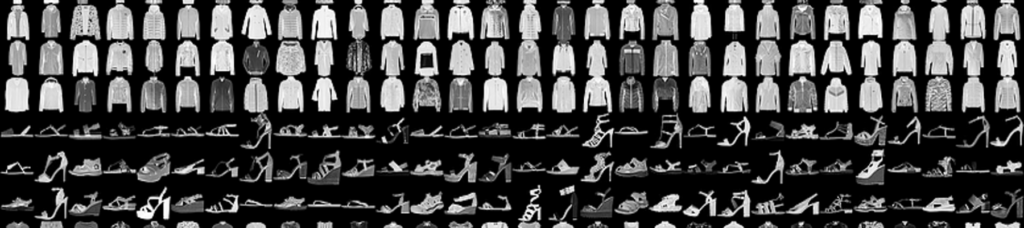
Fashion-MNIST examples
CNN Architecture Design
The network uses three sequential convolutional blocks to extract features hierarchically:
- Block 1 (1 to 32 channels): Captures low-level features such as edges and basic boundaries.
- Block 2 (32 to 64 channels): Combines these edges into local shapes and textures.
- Block 3 (64 to 128 channels): Extracts more complex structural patterns.
Max-pooling layers halve the spatial dimensions after each block, reducing the representation from 28×28 down to 3×3 while the channel depth doubles.
To stabilize training, I applied several design decisions:
- Batch Normalization: I added BatchNorm2d to every convolutional block. Normalizing the activations across the batch kept the gradients stable and improved convergence speed.
- Spatial Dropout (Dropout2d): Standard dropout randomly zeroes out individual pixels. Because neighboring pixels in an image are highly correlated, the network can easily work around pixel-level dropout. I used 2D Spatial Dropout in the convolutional blocks instead. This drops entire feature channels, forcing the network to learn distributed representations rather than relying on specific feature maps.
- Classifier Regularization: After the final convolutional block, the remaining 3×3 feature maps are flattened and passed to a dense layer with 256 units. This fully connected layer is regulated by a 40% dropout rate to reduce overfitting before the final classification layer.
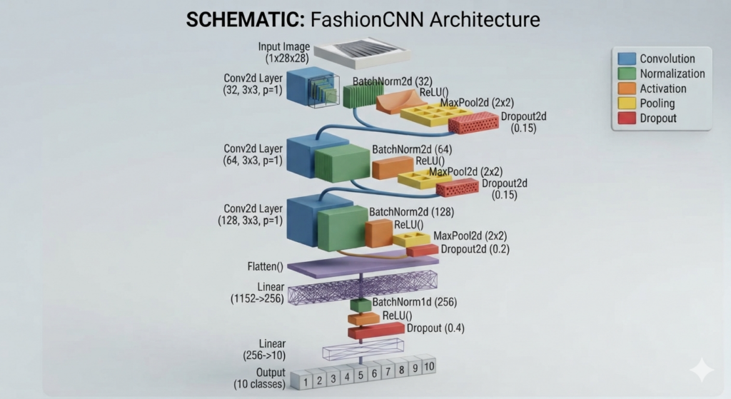
Architecture schematic
Training Configuration
The training setup incorporated several adjustments to improve generalization:
- Data Augmentation: I applied random horizontal flips and minor random rotations (up to 10 degrees) to the training images to make the model less sensitive to slight variations in orientation.
- Optimizer: I used AdamW instead of standard Adam. AdamW decouples weight decay from the gradient updates, which handles L2 regularization more effectively and helps keep the model weights small.
- Learning Rate Schedule: A Cosine Annealing scheduler was used to smoothly decay the learning rate over 15 epochs, helping the model settle into a stable local minimum toward the end of training.
Performance Analysis
To evaluate the model’s performance beyond overall accuracy, I calculated class-specific precision, recall, F1-score, and specificity.
| Class Name | Precision | Recall (Sens) | F1-Score | Specificity |
| T-shirt/top | 0.8745 | 0.8850 | 0.8797 | 0.9859 |
| Trouser | 0.9950 | 0.9870 | 0.9910 | 0.9994 |
| Pullover | 0.8847 | 0.8820 | 0.8833 | 0.9872 |
| Dress | 0.9163 | 0.9410 | 0.9285 | 0.9904 |
| Coat | 0.8673 | 0.8890 | 0.8780 | 0.9849 |
| Sandal | 0.9909 | 0.9750 | 0.9829 | 0.9990 |
| Shirt | 0.7882 | 0.7480 | 0.7676 | 0.9777 |
| Sneaker | 0.9452 | 0.9840 | 0.9642 | 0.9937 |
| Bag | 0.9899 | 0.9850 | 0.9875 | 0.9989 |
| Ankle boot | 0.9836 | 0.9620 | 0.9727 | 0.9982 |
- Overall Accuracy: 92.38%
- Macro Precision: 0.9236
- Macro Recall: 0.9238
- Macro F1-Score: 0.9235
- Macro Specificity: 0.9915
Observations
The class-by-class metrics highlight the specific structural challenges of the dataset:
- Distinct Classes: The model achieved high F1-scores on classes with distinct shapes, such as Trousers (0.9910) and Bags (0.9875).
- Ambiguous Classes: The model struggled most with Shirts (F1-score of 0.7676), which were frequently misclassified as Coats or T-shirts. This is a common issue given the structural overlap between these categories in low-resolution grayscale images.
Analyzing these metrics helped clarify where the 3-block architecture reaches its limits and demonstrated how spatial regularization and data augmentation affect classification performance across similar categories.